Asymmetric Gaussian Fit Function Discontinuity


Hammy
Sun, 03/17/2013 - 06:35 am
I've made an attempt at using a step-function to have the program fit the low-energy tail side of the peak with a modified Gaussian, and then at the point where the shape deviates and begins its Gaussian form, it switches to fitting with a regular Gaussian equation.
The problem I'm seeing is a sort of jump-discontinuity between the end of the modified Gaussian and the beginning of the standard Gaussian fit. I've been trying to figure out a way to fix this, but have been unsuccessful. It's small, though, and only noticeable if zoomed in on the peak. I'll attach a jpeg of one of the graphs, the code, as well as my Igor file.
Thanks.
Function GaussTail (w, x) : FitFunc
// Parameter declaration
Variable x // X coordinate
Wave w // Wave with the coefficient of the fit
// Local variable declaration
Variable bg // Background
Variable tail // Asymmetric Gaussian with low-energy Tail
// w[0] = background slope
// w[1] = background offset
// w[2] = amplitude of peak
// w[3] = peak centroid
// w[4] = Gaussian sigma
// w[5] = Distance below w[3] where shape deviates from Gaussian
// Fitting the Asymmetric Gaussian \\
// The bg should be added to whichever side of the function \\
// exhibits positive background deviation from the other side of \\
// the peak. In the case of Alpha particle spectroscopy, this will \\
// typically be on the low-energy tail side. If the background is \\
// equally offset on both sides, add the bg to both sides of the \\
// function. \\
// Calculate the background
bg = w[0]*x + w[1]
// The fit function will perform a loop which ends once the
// function reaches the X value where the low-energy tail
// ends and the Gaussian begins. A modified form of the
// Gaussian is used in this region (Koskelo et al., 1996):
// f(x) = Ae^(C (2x-2u+C) / (2q^2) ) , for x < u-C, where u is the
// peak centroid, C is the distance from the centroid to the point
// where the Gaussian behavior begins and the tailing ends,
// q is the Gaussian sigma, and A is the amplitude of the peak.
If (x < w[3]-w[5])
tail =bg+ w[2]*exp(w[5]*(2*x-2*w[3]+w[5])/(2*w[4]^2))
// When the fit function reaches the adjoining point of the tail and
// Gaussian, the function continues calculating the fit with the
// following equation: f(x) = Ae^( -((x-u)/(2q))^2 ), which can be
// recognized as a standard Gaussian form. It can be modified
// to use the area under the peak as a parameter in place of
// the amplitude by dividing by q*sqrt(2pi).
Elseif (x >= w[3]-w[5])
tail = w[2]*exp(-(x-w[3])^2/(2*w[4]^2))
Endif
// Returns the combined fit
Return tail
End

Also, try this below. The coding x = test ? yes answer : no answer should be faster than an if ... endif test.
wave w
variable x
variable bg, offset, rgauss, rtail, rtn
offset = w[3] - w[5]
bg = w[0]*x + w[1]
rgauss = w[2]*exp(-(x - w[3])^2/(2*w[4]^2)
rtail = w[2]*exp(w[5]*(2*x - 2*w[3] + w[5])/(2*w[4]^2)
rtn = x < offset ? rtail : rgauss
return (rtn + bg)
end
In addition, my understanding of tails is, they start at a defined point on one side or the other of the peak. In this case, w[3] - w[5] = C, where C is a defined value that in most cases is ZERO. IOW, are you allowing too much variation in the peak definition?
Finally, I would wonder why you are taking this approach? The S/N ~ 3 in your spectrum. This is just at a borderline where reasonable people say they can define a peak, let alone define a peak with any form of asymmetry. IOW, do you have enough confidence that your data supports a tail gaussian? Have you tried comparing the uncertainty budget returned in just a simple gauss with that from your tailed gauss?
--
J. J. Weimer
Chemistry / Chemical & Materials Engineering, UAHuntsville
March 17, 2013 at 01:51 pm - Permalink
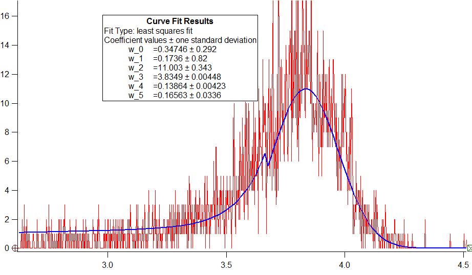
I am not entirely sure if my method was appropriate, but I added the background on the tail side of the peak and did not on the right side, since the left tail is positively offset while the right side of the peak returns to zero. If I have the bg on both sides, then the Gaussian fit extends over a region of nothingness. See below:
Tail side of peak fit
tail =bg+ w[2]*exp(w[5]*(2*x-2*w[3]+w[5])/(2*w[4]^2))
versus Gaussian side of peak,
tail = w[2]*exp(-(x-w[3])^2/(2*w[4]^2))
I'll put this into my file in a little bit, give it a try, and let you know how it works - Thanks.
I'm certainly not an expert on asymmetric Gaussians, but to my understanding, in alpha particle detection it's characteristic of peak shapes due to overlapping. I've tried setting my step parameters to x=w[3] rather than w[3]-w[5], as well as letting w[5] go to zero. The fit function still returns a small value on the range of 0.02 - 0.07, depending on which peak I'm fitting. I've tried what I can think of to try varying ranges of peak definition.
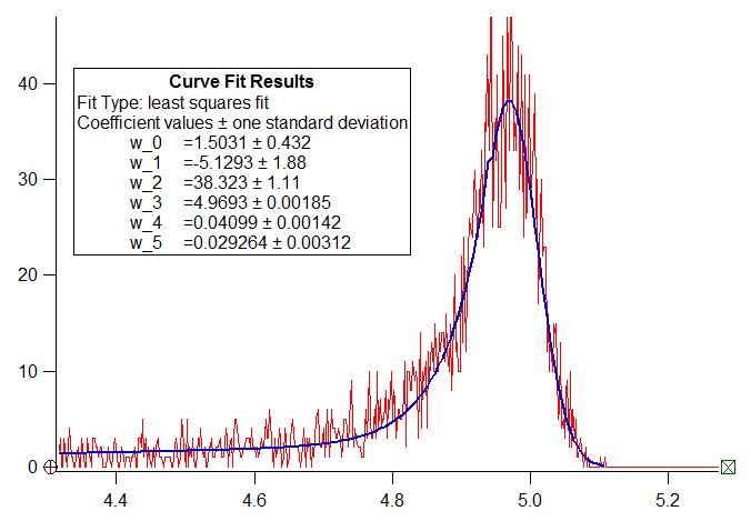
I have also used the regular Gaussian and I do get better fit errors with the modified Gaussian form. The sample was not recorded for long enough to get adequate statistics, unfortunately, so I'm working with what I have. The other peaks that I'm working with are more clearly defined with left-tail asymmetry, as these are all attenuated by various filters of different sizes and material (aluminum, tin, and nickel). I'll attach a jpeg of the nickel attenuation, which shows much better tail-asymmetry since it has more counts than the aluminum, which is shown.
In the nickel attenuated spectrum, the little jagged shape in the Gaussian fit is less exaggerated, which I believe is due to better counting statistics.
Thanks for your response. I'll try some of these ideas out and see how it goes.
March 17, 2013 at 04:01 pm - Permalink
Your background is a linear sloping line. Should it not go from the far left to the far right of the peak regardless of whether the peak has a tail or not? You have not removed the background from the tailed peak, but you do remove it from the normal peak. I suspect that this is why you get the discontinuity that you are seeing at the point where the tail starts.
Thanks for the clarification. I was thinking in spectroscopy terms.
I do find it interesting that this system is to be fit with a tail peak rather than two Gaussians, especially because you say the tail is associated with a "second peak". If the offset of the second peak has a physical meaning that fixes it in position relative to the primary peak, your fitting routine will be more robust using two Gaussian peaks. You will only have the height of the second peak to fit, not its offset. When you use a tail to cover that "second peak", the offset and shape of the tail will change as the height of your second peak changes, even if that second peak stays at the same position relative to the primary peak. So you add one degree of freedom to your system when it really does not warrant having it added.
In mass spectroscopy, this would be equivalent to fitting an isotope peak that is close to the primary peak by one tailed Gaussian peak, even though the position of the isotope peak relative to the primary peak is fixed from first principles.
That is the primary focus of my question.
--
J. J. Weimer
Chemistry / Chemical & Materials Engineering, UAHuntsville
March 18, 2013 at 06:37 am - Permalink
You also mention "MultiPeak2". Are you using the Multipeak Fit 2 package? If so I have two suggestions:
1) It is relatively easy to add a second peak to the left of the main peak using the Add or Edit Peak window. Then you can fit two overlapping peaks. Unfortunately, it is extremely difficult to create a peak picker that will notice the asymmetry and automatically find two peaks there.
2) If the peaks are really asymmetric, that is, the physics of the situation demands asymmetry rather than simply two overlapping peaks, it is possible to use the ExpModGauss peak shape even with left tails, if you have a sufficiently recent version of Igor. You may have to manually set the ExpTau coefficient to a negative number, but the automatic peak picker *should* pick up the asymmetry.
John Weeks
WaveMetrics, Inc.
support@wavemetrics.com
March 18, 2013 at 09:35 am - Permalink
I see the data set that you're trying to fit using Multipeak Fit 2- it is a very nice, clean data set, with just one big peak that seems to require an asymmetric peak. I tried setting that peak to ExpModGauss peak shape. I had to manually change the sign of the ExpTau coefficient. The fit isn't quite as asymmetric as the data.
I have attached a copy of your experiment file with my work in it. I tried three things:
1) Overlapping Gaussian peaks. It took three peaks to adequately fit that tail! That's in MultipeakFit_Set6.
2) ExpModGauss: I had to manually set a negative ExpTau. That peak shape just isn't sufficiently asymmetric. It's in MultipeakFit_Set7.
Then I started playing with anything I could get to match the shape:
3) ExpModGauss plus an additional Lorenzian peak shape overlapping. That's in MultipeakFit_Set8. It's a nice fit, but at this point I've gone well beyond what's justified without some physical explanation!
Remind what sort of data this is?
John Weeks
WaveMetrics, Inc.
support@wavemetrics.com
March 18, 2013 at 09:54 am - Permalink
The original post give a literature reference and equation for an asymmetric peak shape. I get the feeling then that his particular peak shape, rather than just any general asymmetric peak shape, is what is accepted to model the physics of his system.
It may actually be, the tail is to cover a background decay process on one side of the primary peak. Similar things happen with secondary emission off the one side of a primary photoemission peak. Hence, as you note later, the need for three (or more) simple Gaussians in the envelop of the tail.
--
J. J. Weimer
Chemistry / Chemical & Materials Engineering, UAHuntsville
March 18, 2013 at 11:18 am - Permalink
Ah, sure enough. I missed that. I don't have easy access (read: no-cost, and without leaving the office) access to everybody's journals.
But I have to agree with Jeff that the background term is suspect. It's not in the quoted equation included with that reference, and if you disable it, or add it also to the Gaussian, the discontinuity goes away.
I have attached another copy of the experiment that has the background included all the way across, and not included at all, to the Sn_xxx fit. I personally see no compelling reason in that one data set to include the background, and it is clear that the background is the problem. Without background, the peak height isn't quite as good a fit, but removing weighting makes it just as good as the others. But fitting counting data without weighting introduces a bias, as we all know (right?).
John Weeks
WaveMetrics, Inc.
support@wavemetrics.com
March 18, 2013 at 01:00 pm - Permalink
Sorry for the delayed response. I actually tried adding the background to the entire fit, as JJ had suggested and like you already did, and found the same result. I didn't understand clearly enough what the effect would be of having it on one side but not the other. However, I did notice that once I added it to both sides, it did fit the little jagged spot in the peak of the fit, but it did not change the results at all. Not sure why that is, but the fit looks good and Chi^2 looks good.
As far as the "MultiPeak2" package goes, the peak which I was having trouble fitting was the Ni_kev_hist wave, which is identical to the Ni2_kev_hist wave, only slightly shifted left due to lower energy (I haven't labeled the graphs as they were just tests, but it's net counts per energy versus energy).
This is an attenuated alpha particle spectrum from an Americium-241 source measured in a vacuum system with a silicon charged particle detector. The file names are labeled by attenuation (Ni for Nickel, Sn for Tin, Al for Aluminum). The desire was to observe the energy loss of alpha particles as they interact with matter, to determine the stopping power on the charge and velocity. The low-energy tailing can be due to a variety of reasons, but in this case is primarily because of the range over which the alphas are losing energy from interacting with the thickness of the foil (filter/attenuator). So a statistical number of them are interacting with the detector with less energy than their maximum due to multiple interactions prior to hitting the detector, producing a gradual low-energy tail in the spectrum. At least that's the way I understand it, in this case.
The data you fitted in MultiPeak2 was actually my calibration file, where a pulser was used in conjunction with the Am-241 source to determine calibration parameters for the spectra, where the peak you chose was unattenuated and had a much less prominent tail. I should have been a little more explicit when I posted it, but I thought I only loaded the file I was having issues with. If you try to do the MultiPeak2 fitting on the Ni_kev_hist file, you'll see the issue I was running into with MultiPeak2. I've tried it with one, two, and three peaks (by adjusting the threshold), and it always identifies the main peak as negative. But when it tries to fit, it winds up with a straight line down. I've attempted adjusting the fit parameters but haven't had any luck. If I set the width to negative as well as the tau, it fits it perfectly, but no fit results.
I looked in the procedure file and saw mention of something which might relate to what's wrong with it, PeakFunctions2.ipf at the beginning of GaussConvExp section:
if (lwidth > rwidth) // left tail is longer
w[1] = rwidth
w[3] = -3*lwidth // Larry sez: NOTE: ExpGaussian goes wacko if k3 is greater than about 5/k2
else
w[1] = lwidth
w[3] = 3*rwidth // Larry sez: NOTE: ExpGaussian goes wacko if k3 is greater than about 5/k2
endif
Variable widthRatio = abs(w[3])/w[1]
w[2] = height/(1-(widthRatio/(widthRatio+1.2))^2) // totally empirically determined
Would that have anything to do with it, k3 being so large? And I'm running Igor Pro 6.31, by the way.
As far as fitting multiple Gaussians goes, that's the ultimate goal, to deconvolve the peaks when they are present. The source in my file doesn't really exhibit that behavior, of overlapping peaks, but there are other sources which do. The equation I quoted in my function comments is one which is commonly used for fitting the net counts of the asymmetry, though the method that MultiPeak2 uses is more along the lines of what's used by some alpha spectroscopy programs.
I appreciate you both taking a look into my files and errors for me. I'll see what I can find as far as other fitting methods go. This is a good excuse for me to work on my programming, as well as do something useful.
March 19, 2013 at 03:23 pm - Permalink
-Ham
March 19, 2013 at 03:39 pm - Permalink
I am otherwise glad to hear that you are making progress.
As a note ... deconvolution and peak fitting are technically not the same thing. Deconvolution separates a peak in to its convolved components, and peak fitting separates a peak in to its summed components. When you put two or more peaks under one peak, you are doing peak fitting, not peak deconvolution.
(this was an insight that I garnered from an ACS conference many, many years ago)
--
J. J. Weimer
Chemistry / Chemical & Materials Engineering, UAHuntsville
March 19, 2013 at 04:08 pm - Permalink
As far as deconvolution goes, I'm still reading and learning more about it. But from what I've seen, the various equations and stepping functions with modified gaussians to fit these sort of peaks seem to tie right in with doing a deconvolution after doing the sum fit (convolution?). I'm somewhat familiar with convolution theorem as far as Fourier transforms go, so thinking about it that way it kind of makes sense with what you're saying.
March 19, 2013 at 05:45 pm - Permalink
Summing a set of peaks to fit under a single peak is still peak fitting, not convolution.
In spectroscopy, deconvolution is typically used to remove an instrument transform function from a measured spectrum to obtain a true spectrum. Before you start, you must know the exact nature of the instrument transform function. After you are done, you have a a true spectrum. An example is to blur a perfect image with a distorted-focus lens. To recover the perfect image, you have to know the exact nature of how the lens blurs any and all images. Then, you can remove that well-defined blur function from your distorted images that have been captured using the lens.
My experience is, deconvolution should be done before peak fitting, and deconvolution requires a spectrum with a S/N that is greater than what you would use otherwise just for peak fitting.
--
J. J. Weimer
Chemistry / Chemical & Materials Engineering, UAHuntsville
March 20, 2013 at 07:55 am - Permalink
If you think of the peaks as representing impulses that have been broadened by some process or instrument response then the peak fitting is a form of convolution, as you can reconstruct the original impulse (location and intensity) from the fitted peaks.
But I wouldn't want to say it in public :)
I will look into the ExpModGauss function. It really should allow left-tailed peaks.
John Weeks
WaveMetrics, Inc.
support@wavemetrics.com
March 20, 2013 at 01:06 pm - Permalink
John Weeks
WaveMetrics, Inc.
support@wavemetrics.com
March 20, 2013 at 01:33 pm - Permalink