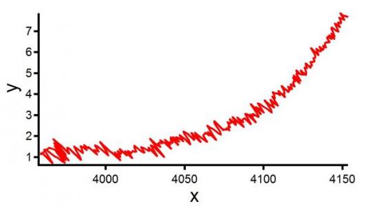
How to apply curve fitting with a model where y shows up on both sides of the equation?

yuzhongbo
Fri, 04/06/2012 - 09:30 pm


Fri, 04/06/2012 - 09:30 pm

Think of your equation as a function Yourfunc(W,x). The inside of the function will likely use the
FindRootsoperation to return y given x and initial guesses of coefficients a,b,c (elements of W). The hardest part will be theFindRootsoperation needs lower and upper bounds (/L and /H flags), and you need to come up with an algorithm that sets these bounds as a function of x, and W. But your function is pretty simple, so that should be doable.HTH,
John Bechhoefer
April 7, 2012 at 08:42 am - Permalink
April 7, 2012 at 09:29 am - Permalink
Instead of:
y=a*(((4*(1-x/b+y/c))^-2)-0.25+x/b-y/c)
I create
G=a*(((4*(1-x/b+y/c))^-2)-0.25+x/b-y/c)-Y (I subtract Y from both sides and make a new dependent variable, G)
I then set G(x) equal to 0 and then find the roots.
April 7, 2012 at 03:41 pm - Permalink
I suggest you use the implicit curve fitting method described in the Manual on PP. III-211,212. In this case, you might have to create an x-wave first, and then apply the methods there. Note that is there a minor typo (missing left brace) on line 15, p. III-212. Also, check the Help file for FuncFit; the information is given there as well. I believe your implicit fitting function would take the form:
Wave w
Variable x
Variable y
//CurveFitDialog/
//CurveFitDialog/ Coefficients 3
//CurveFitDialog/ w[0] = a
//CurveFitDialog/ w[1] = b
//CurveFitDialog/ w[2] = c
return w[0]*(((4*(1-x/w[1]+y/w[2]))^-2)-0.25+x/w[1]-y/w[2])-y
End
April 8, 2012 at 06:24 am - Permalink
April 8, 2012 at 07:54 am - Permalink
WAVE waveX, waveY
Duplicate/O waveX, waveXFit, waveYFit
Make/D/O FitCoefs={4e-6,1.6e4,5e-5} // a, b, c
FuncFit/ODR=3 FitCurve, FitCoefs /X={waveX, waveY}/XD={waveXFit,waveYFit}
end
and got the following result (with attached graph)
Fit converged properly
FitCoefs={-6.9236e-006,15941,6.9236e-006}
V_chisq= 3.61961e-024;V_npnts= 296;V_numNaNs= 0;V_numINFs= 0;
W_sigma={2.45e-16,9.78e-07,2.45e-16}
Coefficient values ± one standard deviation
a =-6.9236e-006 ± 2.45e-016
b =15941 ± 9.78e-007
c =6.9236e-006 ± 2.45e-016
However, I noticed that the 'a' and 'c' coefficients were very sensitive to initial guesses, so I would not trust their values. Notice the 'coincidental' agreement of their magnitudes, but with opposite signs. I don't know what this indicates about your model.
April 8, 2012 at 10:01 am - Permalink
April 8, 2012 at 12:04 pm - Permalink
A result in which various different sets of coefficients can result in similarly good fits usually indicates "identifiability" problems. In fact, the fit that Steve Chinn got looks too good to be true; I'm not sure what coefficients you used to get the smooth line in your graph.
Identifiability problems means that two or more of the fit coefficients trade off in a way that makes it nearly impossible to solve for the values of both at once. They are correlated in a way that if you adjust one, you can find a value of the other that makes a fit that is nearly as good. Identifiability problems are generally accompanied by large estimated errors on the fit coefficients; that doesn't seem to be the case here. I don't know why.
You can diagnose identifiability problems after a successful fit by looking at the correlation matrix. To learn how to get it from an Igor fit execute this command on the command line:
DisplayHelpTopic "Correlation matrix"
It requires that you use the /M=2 flag with FuncFit. Adding /M=2 right after the FuncFit keyword in Steve's FitIt() function I made a correlation matrix for the fit. Here it is:
1 -0.578566 -1
-0.578566 1 0.578565
-1 0.578565 1
Note the off-diagonal values of -1. That indicates essentially perfect correlation between w[0] and w[2]. Looking at your equation, it doesn't appear that there is a true mathematical dependence, but it looks like within the domain of the data, there is little to distinguish a and c.
Unfortunately, this is not a problem with Igor's fitting routines. It is a mathematical problem that can only be solved by either figuring out how to get data that will distinguish those coefficients, or by simplifying your fit function.
John Weeks
WaveMetrics, Inc.
support@wavemetrics.com
April 9, 2012 at 04:35 pm - Permalink
Wave w
Variable x
Variable y
//CurveFitDialog/
//CurveFitDialog/ Coefficients 3
//CurveFitDialog/ w[0] = a
//CurveFitDialog/ w[1] = b
//CurveFitDialog/ w[2] = c
Variable term1 = (4*(1-x/w[1]+y/w[2]))^-2
Variable term2 = x/w[1]
Variable term3 = y/w[2]
print x, y, term1, term2, term3
return w[0]*((term1)-0.25+term2-term3)-y
End
This makes the function pretty useless for fitting because priting all those numbers in the history slows it down so much. But the result was quite instructive. Here is a little bit of the output:
4137.8 6.3 3.93671e-12 0.258612 126000
4139.6 6.23 4.02568e-12 0.258725 124600
4138.94 6.37 3.85067e-12 0.258684 127400
4139.07 6.44 3.76741e-12 0.258692 128800
4139.69 6.47 3.73256e-12 0.258731 129400
4140.65 6.47 3.73256e-12 0.258791 129400
Note that term1 is many orders of magnitude smaller than the rest of the numbers, and term2 is quite a bit smaller than term3, so most of the contribution to the output value comes from just term3. That means that there is little contribution to the result from coefficient b and in term3 the result is determined by a ration of a/c, so as long as a and c are adjusted to keep a/c constant, you will get almost the identical fit.
John Weeks
WaveMetrics, Inc.
support@wavemetrics.com
April 9, 2012 at 04:55 pm - Permalink
IF one accepts the premise that a hidden correlation forces a = -c, then the original equation from yuzhongbo simplifies to the extent that there is an explicit, rather than implicit, relation among the variables (if I have done the math right).
Wave w
Variable x
//CurveFitDialog/ These comments were created by the Curve Fitting dialog. Altering them will
//CurveFitDialog/ make the function less convenient to work with in the Curve Fitting dialog.
//CurveFitDialog/ Equation:
//CurveFitDialog/ f(x) = c*( 0.5/sqrt(1-4*x/b) + x/b -1 )
//CurveFitDialog/ End of Equation
//CurveFitDialog/ Independent Variables 1
//CurveFitDialog/ x
//CurveFitDialog/ Coefficients 2
//CurveFitDialog/ w[0] = b
//CurveFitDialog/ w[1] = c
return w[1]*( 0.5/sqrt(1-4*(x/w[0])) + (x/w[0]) -1 )
End
The resulting explicit fit gives the following results and attached graph.
fit_waveY= fitcurve(w_coef,x)
w_coef={16651,0.99155}
V_chisq= 72.5424;V_npnts= 296;V_numNaNs= 0;V_numINFs= 0;
V_startRow= 0;V_endRow= 295;
W_sigma={2.31,0.0148}
Coefficient values ± one standard deviation
b =16651 ± 2.31
c =0.99155 ± 0.0148
I would suggest that the original fitting model warrants re-examination.
April 10, 2012 at 10:40 am - Permalink
May 4, 2012 at 08:45 am - Permalink